Jupyter Notebook: Plotting Sea Surface Temperature Anomalies (SSTA)

Load Libraries

%config IPCompleter.greedy = True
# ignore warnings

import os
import warnings
warnings.filterwarnings("ignore")

import numpy as np
import xarray as xr
from statsmodels.tsa.tsatools import detrend

import matplotlib
import matplotlib.pyplot as plt
import matplotlib.cm as mpl_cm
from matplotlib.backends.backend_pdf import PdfPages # one pdf multipage

import cartopy.crs as ccrs
from cartopy.mpl.ticker import LatitudeFormatter, LongitudeFormatter
from shapely.geometry.polygon import LinearRing

## my_pylibs using PYTHONPATH
from climatology import month_to_djf, detrend_3d

R_nino3  = LinearRing(list(zip([210-360, 210-360, 270-360, 270-360], [-5, 5, 5, -5])))
R_nino4  = LinearRing(list(zip([160, 160, 210, 210], [-5, 5, 5, -5])))
R_nino34 = LinearRing(list(zip([190-360, 190-360, 240-360, 240-360], [-5, 5, 5, -5])))
R_nino12 = LinearRing(list(zip([270-360, 270-360, 280-360, 280-360], [-10, 0, 0, -10])))
R_IODW   = LinearRing(list(zip([50, 50, 70, 70], [-10, 10, 10, -10])))
R_IODE   = LinearRing(list(zip([90, 90, 110, 110], [-10, 0, 0, -10])))
R_ALT3   = LinearRing(list(zip([340-360, 340-360, 360-360, 360-360], [-3, 3, 3, -3])))
R_NAT    = LinearRing(list(zip([320-360, 320-360, 340-360, 340-360], [5, 20, 20, 5])))

Calculate Monthly Anomalies Using Xarray

sst_file = "/share/kkraid/zhaos/data/sst/ersst/sst.mnmean.nc"
xr_sst   = xr.open_dataset(sst_file)["sst"][:, ::-1, :] ## latitude is revsered in ersst

## remove the climatology of 1921 to 1980
sst_c = xr_sst.sel(time=slice('1981', '2010')).groupby('time.month').mean('time')
sst_a = xr_sst.groupby('time.month') - sst_c

Calculate Detrended Anomalies

sst_ad = detrend_3d(sst_a, order=2)

Calculate Seasonal DJF Anomalies

djfsst_a  = month_to_djf(sst_a)
djfsst_ad = month_to_djf(sst_ad)

Setting Plot Axis and Levels

## x and y axes
lon = sst_a.lon
lat = sst_a.lat

## fill levels
sst_fill = np.arange(-3, 3.01, step=0.5)

## projections for data and target
data_crs = ccrs.PlateCarree(central_longitude=0)
tar_crs  = ccrs.Mollweide(central_longitude=200)

nrow = 15
ncol = 10
fig, axs = plt.subplots(nrow, ncol,  figsize=(2.25*ncol, 1.605 * nrow), subplot_kw={'projection': tar_crs} )
for i, ax in enumerate( axs.flatten() ):
    sel_year = 1871 + i
    imag0 = ax.contourf(lon, lat, djfsst_a.sel(year=sel_year), extend = 'both', levels = sst_fill, cmap = plt.cm.RdBu_r, transform=data_crs)
    ax.coastlines(alpha=0.5)
    ax.add_geometries([R_nino34], crs=data_crs, facecolor='none', edgecolor='gray', linewidth=0.5, linestyle='dashed')
    ax.add_geometries([R_IODW, R_IODE], crs=data_crs, facecolor='none', edgecolor='gray', linewidth=0.5, linestyle='dashed')
    ax.set_title( '{0}/{1} DJF'.format(sel_year-1, sel_year) )

fig.colorbar(imag0, ax=axs.flatten(), orientation='horizontal', shrink=0.5, aspect=30, pad = 0.01)
fig.text(0.89, 0.91, '@SenZhao', fontsize=16, color='darkorange', va='center', ha='right')
fig.suptitle('DJF SST anomaly for 1871-2020 derived from ERSST', y=0.91, fontsize=20, fontweight='bold')
fig.savefig('figures/sstdjf_multiples_ersst_1871-2020.png', dpi = 200, bbox_inches='tight', pad_inches = 0.5)

# pdf = PdfPages('figures/sstdjf_multiples_ersst_1871-2020.pdf')
# pdf.savefig(fig, bbox_inches='tight', dpi=480)
# pdf.close()

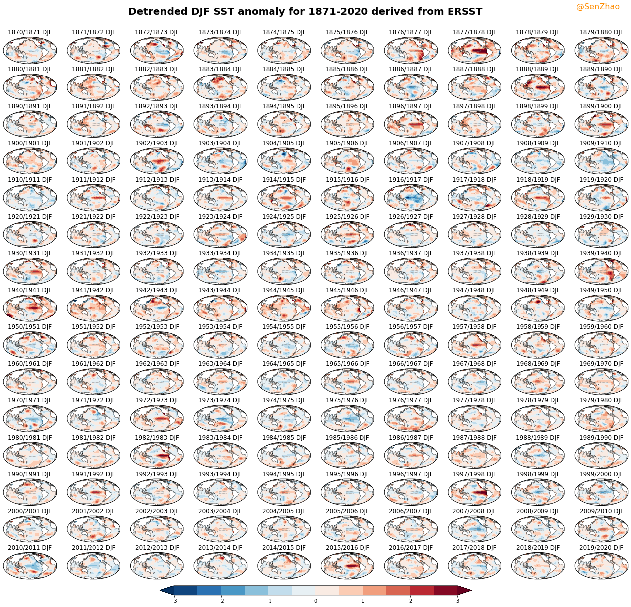
nrow = 15
ncol = 10
fig, axs = plt.subplots(nrow, ncol,  figsize=(2.25*ncol, 1.605 * nrow), subplot_kw={'projection': tar_crs} )
for i, ax in enumerate( axs.flatten() ):
    sel_year = 1871 + i
    imag0 = ax.contourf(lon, lat, djfsst_ad.sel(year=sel_year), extend = 'both', levels = sst_fill, cmap = plt.cm.RdBu_r, transform=data_crs)
    ax.coastlines(alpha=0.5)
    ax.add_geometries([R_nino34], crs=data_crs, facecolor='none', edgecolor='gray', linewidth=0.5, linestyle='dashed')
    ax.add_geometries([R_IODW, R_IODE], crs=data_crs, facecolor='none', edgecolor='gray', linewidth=0.5, linestyle='dashed')
    ax.set_title( '{0}/{1} DJF'.format(sel_year-1, sel_year) )

fig.colorbar(imag0, ax=axs.flatten(), orientation='horizontal', shrink=0.5, aspect=30, pad = 0.01)
fig.text(0.89, 0.91, '@SenZhao', fontsize=16, color='darkorange', va='center', ha='right')
fig.suptitle('Detrended DJF SST anomaly for 1871-2020 derived from ERSST', y=0.91, fontsize=20, fontweight='bold')
fig.savefig('figures/detrend_sstdjf_multiples_ersst_1871-2020.png', dpi = 200, bbox_inches='tight', pad_inches = 0.5)

# pdf = PdfPages('figures/detrend_sstdjf_multiples_ersst_1871-2020.pdf')
# pdf.savefig(fig, bbox_inches='tight', dpi=480)
# pdf.close()