Does Off-Equatorial South Pacific Heat Content Really Provide Additional Predictive Skill of ENSO Beyond the Equatorial Pacific Heat Content?
Comments on Yang et al. (2025)
Yang et al. (2025) proposed that off-equatorial South Pacific (SP) sea surface height (SSH)—a proxy for heat content—can enhance ENSO prediction skill at lead times beyond 9 months, based on a Linear Inverse Model (LIM) framework. They constructed two LIM configurations:
- Full LIM: Includes 20 leading principal components (PCs) of tropical Pacific SST and the monthly SP SSH index, resulting in 21 degrees of freedom.
- No-SP SSH LIM: Contains only the 20 SST PCs, but uses the dynamical operators (Green’s function) derived from the Full LIM.
By comparing the predictive skill of these two LIMs, they attributed the improved skill of the Full LIM at long lead times to the inclusion of SP SSH.
However, this method of testing may be insufficient to establish a causal or mechanistic role of off-equatorial SP heat content in enhancing ENSO predictability. While heat content is well known to be important for ENSO prediction—both from theoretical frameworks like the Recharge Oscillator theory (Jin 1997) and from observational analyses such as Meinen and McPhaden (2000)—it remains unclear whether the added skill comes from the off-equatorial region or simply reflects better representation of equatorial Pacific warm water volume.
Moreover, earlier LIM and RO-based studies already showed that equatorial heat content plays a central role in ENSO evolution, raising the question: does SP SSH truly provide additional, independent skill?
Is Off-Equatorial SP SSH Really an Independent Predictor Beyond the establised extended nonlinear RO (XRO)?
The central question remains: Does off-equatorial SP SSH truly provide additional ENSO predictability beyond what is captured in equatorial dynamics and known interbasin feedbacks?
Our recent work, Zhao et al. (2024), shows that ENSO predictability can be substantially enhanced when considering a physically interpretable and explainable framework like the eXtended nonlinear Recharge Oscillator (XRO). The XRO builds on core RO dynamics and explicitly includes interactions with other climate modes.
So if the added SP SSH helps prediction, is it doing so independently, or is it just capturing signals already embedded in the equatorial or interbasin interactions that XRO accounts for?
In this notebook, we would inverstigate these above questions. We will use the same dataset ORAS5 and definition of off-equatorial SP SSH (18°S–14°S, 150°E–135°W) as in Yang et al. (2025).
References
- Yang, G., Jin, Y., Zhao, Y., Di Lorenzo, E., McPhaden, M. J., & Lin, X. (2025). Improving ENSO Prediction at Longer Lead Times: Role of Off-Equatorial South Pacific Heat Content. Geophysical Research Letters, 52(14), e2024GL114540.
- Zhao, S., Jin, F.-F., Stuecker, M. F., Thompson, P. R., Kug, J.-S., McPhaden, M. J., et al. (2024). Explainable El Niño predictability from climate mode interactions. Nature, 630(8018), 891–898.
- Meinen, C. S., & McPhaden, M. J. (2000). Observations of Warm Water Volume Changes in the Equatorial Pacific and Their Relationship to El Niño and La Niña. Journal of Climate, 13(20), 3551–3559.
- Jin, F.-F. (1997). An Equatorial Ocean Recharge Paradigm for ENSO. Part I: Conceptual Model. Journal of the Atmospheric Sciences, 54(7), 811–829.
%config IPCompleter.greedy = True
%matplotlib inline
%config InlineBackend.figure_format='retina'

%load_ext autoreload
%autoreload 2

import warnings
warnings.filterwarnings("ignore")

import os
import glob

import numpy  as np
import xarray as xr

import statsmodels.api as sm

import matplotlib
import matplotlib.cm as cm
import matplotlib.pyplot as plt

import senpy as sp
from senpy.Xeof import eof_analysis, plot_eofs, plot_pcs
from senpy.XRO import XRO

plt.style.use("science")
Data Processing
ORAS5 data loading
oras5_ds = sp.ORA_onemodel_vars(model='oras5', vars=['sst', 'ssh', 'd20'], time_slice=slice('1958-01', '2024-12')).load()
oras5_a = oras5_ds.clim.anomalies(clim_slice=slice('1958-01', '2024-12'))
oras5_a = oras5_a.detrend(order=2).compute()
oras5_ds.close()
ORAS5 climate indices
ssti_ds = sp.global_sst_indices(oras5_a.sst)
sshi_ds = sp.tropical_WWVs(oras5_a.ssh)
d20i_ds = sp.tropical_WWVs(oras5_a.d20)
SST leading 20 EOFs and PCs
eof_ds, pc_ds, vfrac_ds = eof_analysis(oras5_a.sst.sel(lat=slice(-30, 30), lon=slice(130, 290)), neof=20)
# fig_eofs = plot_eofs(eofs=eof_ds, vfracs=vfrac_ds, lon_0=200, ncol=5, figsize=(15, 6), maxval=0.3)
# fig_pcs = plot_pcs(pcs=pc_ds, vfracs=vfrac_ds, ncol=5, figsize=(13, 6))
Note: If you take a look at the EOFs and PCs of higher modes (large than 5), you have no idea about the physical meaning and time scale is very noisey.
XRO model and forecasts
XRO state vectors
index_a_ssh = xr.merge([ssti_ds, sshi_ds]).rename({'Hm': 'WWV', 'SASD2': 'SASD'})
index_a_d20 = xr.merge([ssti_ds, d20i_ds]).rename({'Hm': 'WWV', 'SASD2': 'SASD'})

RO_vars = ['Nino34', 'WWV']
XRO_vars = ['Nino34', 'WWV', 'NPMM', 'SPMM', 'IOB', 'IOD', 'SIOD', 'TNA', 'ATL3', 'SASD']
RO_SPSSH_vars = ['Nino34', 'WWV', 'Hsw_Yang25']
XRO_SPSSH_vars = ['Nino34', 'WWV', 'NPMM', 'SPMM', 'IOB', 'IOD', 'SIOD', 'TNA', 'ATL3', 'SASD', 'Hsw_Yang25']

index_RO_a_ssh = index_a_ssh[RO_vars]
index_RO_SPSSH_a_ssh = index_a_ssh[RO_SPSSH_vars]
index_XRO_a_ssh = index_a_ssh[XRO_vars]
index_XRO_SPSSH_a_ssh = index_a_ssh[XRO_SPSSH_vars]
XRO trainning and reforecasts
XRO_model = XRO(ncycle=12, ac_order=2) # here we use the stardard version of XRO with annual cycle and semi-annual cycle
maskNT = ['T2', 'TH'] # as in Zhao et al. 2024, T**2 and T*H nonlinearity in ENSO SST equation
maskNH = []
maskb = ['IOD']
n_month = 12

fit_RO = XRO_model.fitbcNRO_matrix(index_RO_a_ssh, maskNT = maskNT, maskNH = maskNH)
fcst_RO = XRO_model.reforecast(fit_ds=fit_RO, init_ds=index_RO_a_ssh, n_month=n_month, noise_type='zero')

fit_RO_SPSSH = XRO_model.fitbcNRO_matrix(index_RO_SPSSH_a_ssh, maskNT = maskNT, maskNH = maskNH)
fcst_RO_SPSSH = XRO_model.reforecast(fit_ds=fit_RO_SPSSH, init_ds=index_RO_SPSSH_a_ssh, n_month=n_month, noise_type='zero')

fit_XRO = XRO_model.fitbcNRO_matrix(index_XRO_a_ssh, maskNT = maskNT, maskNH = maskNH, maskb=maskb)
fcst_XRO = XRO_model.reforecast(fit_ds=fit_XRO, init_ds=index_XRO_a_ssh, n_month=n_month, noise_type='zero')

fit_XRO_SPSSH = XRO_model.fitbcNRO_matrix(index_XRO_SPSSH_a_ssh, maskNT = maskNT, maskNH = maskNH, maskb=maskb)
fcst_XRO_SPSSH = XRO_model.reforecast(fit_ds=fit_XRO_SPSSH, init_ds=index_XRO_SPSSH_a_ssh, n_month=n_month, noise_type='zero')
skillAC_RO = sp.calc_forecast_skill(fcst_RO, index_RO_a_ssh, by_month=True)
skillAC_XRO = sp.calc_forecast_skill(fcst_XRO, index_XRO_a_ssh, by_month=True)
skillAC_RO_SPSSH = sp.calc_forecast_skill(fcst_RO_SPSSH, index_RO_SPSSH_a_ssh, by_month=True)
skillAC_XRO_SPSSH = sp.calc_forecast_skill(fcst_XRO_SPSSH, index_XRO_SPSSH_a_ssh, by_month=True)
corr_cdict = sp.cmap.dict_cmap_contourf(levels=np.arange(0, 1.01, step=0.05), name='RdBu_r', extend='neither')
corrD_cdict = sp.cmap.dict_cmap_contourf(levels=np.arange(-0.21, 0.211, step=0.03), mid=True, extend='neither')
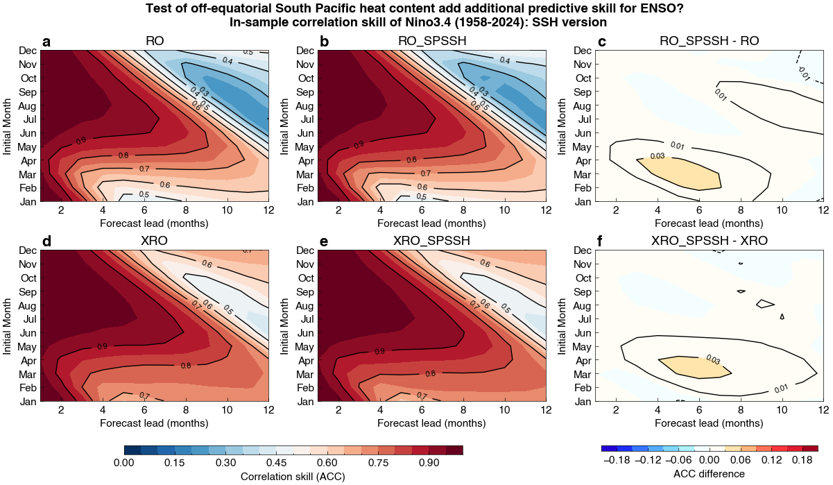
fig, axes = plt.subplots(2, 3, figsize=(12, 7), layout='compressed')
sel_var = 'Nino34'
group_ds = [ skillAC_RO[sel_var], skillAC_RO_SPSSH[sel_var], skillAC_XRO[sel_var], skillAC_XRO_SPSSH[sel_var] ]
group_title = ['RO', 'RO_SPSSH', 'XRO', 'XRO_SPSSH']
for i, ax in enumerate(axes[0:2, 0:2].flat):
g_ds = group_ds[i]
imag = ax.contourf(g_ds.lead, g_ds.month, g_ds, **corr_cdict)
cs = ax.contour(g_ds.lead, g_ds.month, g_ds, levels=np.arange(0, 1, step=0.1), colors='k',)
ax.clabel(cs, inline=True, fontsize=8, fmt='%1.1f')
ax.set_title(group_title[i])
cbar = fig.colorbar(imag, ax=axes[0:2, 0:2], orientation='horizontal', aspect=40, shrink=0.67)
cbar.set_label("Correlation skill (ACC)")
diff_ds = [ skillAC_RO_SPSSH[sel_var] - skillAC_RO[sel_var], skillAC_XRO_SPSSH[sel_var] - skillAC_XRO[sel_var] ]
diff_title = ['RO_SPSSH - RO', 'XRO_SPSSH - XRO']
for i, ax in enumerate(axes[:, 2].flat):
g_ds = diff_ds[i]
imagD = ax.contourf(g_ds.lead, g_ds.month, g_ds, **corrD_cdict)
cs = ax.contour(g_ds.lead, g_ds.month, g_ds, levels=np.arange(-0.19, 0.2, step=0.02), colors='k',)
ax.clabel(cs, inline=True, fontsize=8, fmt='%1.2f')
ax.set_title(diff_title[i])
cbarD = fig.colorbar(imagD, ax=axes[:, 2], orientation='horizontal', aspect=40, shrink=0.95)
cbarD.set_label("ACC difference")
for ax in axes.flat:
sp.set_monticks(ax, axis='y', option=1)
ax.set_ylabel('Initial Month')
ax.set_xlabel('Forecast lead (months)')
ax.set_xlim([1, 12])
fig.suptitle("Test of off-equatorial South Pacific heat content add additional predictive skill for ENSO? \n In-sample correlation skill of Nino3.4 (1958-2024): SSH version", fontweight='bold', fontsize='large')
sp.set_legend_alphabet(fig, axes.flat)
sp.savefig(fig, fname='fig_comment_Yang25_GRL_ENSO_skill_SP_SSH.png')
XRO versions with heat content using D20
index_RO_a_d20 = index_a_d20[RO_vars]
index_RO_SPSSH_a_d20 = index_a_d20[RO_SPSSH_vars]
index_XRO_a_d20 = index_a_d20[XRO_vars]
index_XRO_SPSSH_a_d20 = index_a_d20[XRO_SPSSH_vars]

fit1_RO = XRO_model.fitbcNRO_matrix(index_RO_a_d20, maskNT = maskNT, maskNH = maskNH)
fcst1_RO = XRO_model.reforecast(fit_ds=fit1_RO, init_ds=index_RO_a_d20, n_month=n_month, noise_type='zero')

fit1_RO_SPSSH = XRO_model.fitbcNRO_matrix(index_RO_SPSSH_a_d20, maskNT = maskNT, maskNH = maskNH)
fcst1_RO_SPSSH = XRO_model.reforecast(fit_ds=fit1_RO_SPSSH, init_ds=index_RO_SPSSH_a_d20, n_month=n_month, noise_type='zero')

fit1_XRO = XRO_model.fitbcNRO_matrix(index_XRO_a_d20, maskNT = maskNT, maskNH = maskNH, maskb=maskb)
fcst1_XRO = XRO_model.reforecast(fit_ds=fit1_XRO, init_ds=index_XRO_a_d20, n_month=n_month, noise_type='zero')

fit1_XRO_SPSSH = XRO_model.fitbcNRO_matrix(index_XRO_SPSSH_a_d20, maskNT = maskNT, maskNH = maskNH, maskb=maskb)
fcst1_XRO_SPSSH = XRO_model.reforecast(fit_ds=fit1_XRO_SPSSH, init_ds=index_XRO_SPSSH_a_d20, n_month=n_month, noise_type='zero')

skillAC1_RO = sp.calc_forecast_skill(fcst1_RO, index_RO_a_d20, by_month=True)
skillAC1_XRO = sp.calc_forecast_skill(fcst1_XRO, index_XRO_a_d20, by_month=True)
skillAC1_RO_SPSSH = sp.calc_forecast_skill(fcst1_RO_SPSSH, index_RO_SPSSH_a_d20, by_month=True)
skillAC1_XRO_SPSSH = sp.calc_forecast_skill(fcst1_XRO_SPSSH, index_XRO_SPSSH_a_d20, by_month=True)
corr_cdict = sp.cmap.dict_cmap_contourf(levels=np.arange(0, 1.01, step=0.05), name='RdBu_r', extend='neither')
corrD_cdict = sp.cmap.dict_cmap_contourf(levels=np.arange(-0.21, 0.211, step=0.03), mid=True, extend='neither')
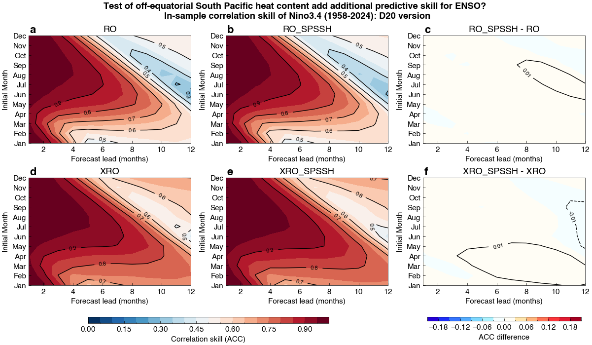
fig, axes = plt.subplots(2, 3, figsize=(12, 7), layout='compressed')
sel_var = 'Nino34'
group_ds = [ skillAC1_RO[sel_var], skillAC1_RO_SPSSH[sel_var], skillAC1_XRO[sel_var], skillAC1_XRO_SPSSH[sel_var] ]
group_title = ['RO', 'RO_SPSSH', 'XRO', 'XRO_SPSSH']
for i, ax in enumerate(axes[0:2, 0:2].flat):
g_ds = group_ds[i]
imag = ax.contourf(g_ds.lead, g_ds.month, g_ds, **corr_cdict)
cs = ax.contour(g_ds.lead, g_ds.month, g_ds, levels=np.arange(0, 1, step=0.1), colors='k',)
ax.clabel(cs, inline=True, fontsize=8, fmt='%1.1f')
ax.set_title(group_title[i])
cbar = fig.colorbar(imag, ax=axes[0:2, 0:2], orientation='horizontal', aspect=40, shrink=0.67)
cbar.set_label("Correlation skill (ACC)")
diff_ds = [ skillAC1_RO_SPSSH[sel_var] - skillAC1_RO[sel_var], skillAC1_XRO_SPSSH[sel_var] - skillAC1_XRO[sel_var] ]
diff_title = ['RO_SPSSH - RO', 'XRO_SPSSH - XRO']
for i, ax in enumerate(axes[:, 2].flat):
g_ds = diff_ds[i]
imagD = ax.contourf(g_ds.lead, g_ds.month, g_ds, **corrD_cdict)
cs = ax.contour(g_ds.lead, g_ds.month, g_ds, levels=np.arange(-0.19, 0.2, step=0.02), colors='k',)
ax.clabel(cs, inline=True, fontsize=8, fmt='%1.2f')
ax.set_title(diff_title[i])
cbarD = fig.colorbar(imagD, ax=axes[:, 2], orientation='horizontal', aspect=40, shrink=0.95)
cbarD.set_label("ACC difference")
for ax in axes.flat:
sp.set_monticks(ax, axis='y', option=1)
ax.set_ylabel('Initial Month')
ax.set_xlabel('Forecast lead (months)')
ax.set_xlim([1, 12])
fig.suptitle("Test of off-equatorial South Pacific heat content add additional predictive skill for ENSO? \n In-sample correlation skill of Nino3.4 (1958-2024): D20 version", fontweight='bold', fontsize='large')
sp.set_legend_alphabet(fig, axes.flat)
sp.savefig(fig, fname='fig_comment_Yang25_GRL_ENSO_skill_SP_D20.png')
Results and Discussion
The results presented here indicate that off-equatorial South Pacific (SP) heat content (SSH or D20) does not significantly provide additional ENSO predictability beyond what is already captured by equatorial Pacific recharge dynamics and known interbasin feedbacks, such as interactions with the Indian Ocean and Atlantic SST modes as represented in models like the eXtended nonlinear Recharge Oscillator (XRO).
This suggests that the predictive signal in off-equatorial South Pacific heat content (SSH) may not be an independent source of ENSO skill, but rather reflects variability that is already encoded in equatorial and interbasin predictors.